녹지, 수계, 도로 추가하기

개요

행정구역 경계만 표시된 지도는 때로는 너무 단조롭게 보일 수 있습니다. 이를 개선하기 위해 산지, 녹지, 수계, 도로 등의 정보를 추가하여 더 풍성한 지도를 만드는 방법을 소개합니다. 이번 글에서는 행정구역 경계에 다양한 지형 데이터를 병합해 시각화하는 과정을 설명합니다.

데이터 다운로드

먼저 필요한 데이터를 다운로드합니다. 행정구역 경계, 산지, 녹지, 수계, 도로 데이터는 V-World 디지털트윈국토에서 다운받을 수 있습니다. 모든 데이터의 좌표계는 GRS80(EPSG:5186)으로 동일하기 때문에 좌표계를 일치시키는 추가 작업은 필요하지 않습니다.

데이터	게시물	좌표계
행정구역 경계	행정구역시군구_경계	GRS80(EPSG:5186)
산지	(연속주제)_산지관리/보전준보전산지	GRS80(EPSG:5186)
녹지	(연속주제)_국토계획/공간시설	GRS80(EPSG:5186)
수계	실폭하천	GRS80(EPSG:5186)
도로	(도로명주소)실폭도로	GRS80(EPSG:5186)

데이터 로드 및 병합

다운로드한 데이터 파일을 불러와 병합합니다. 먼저 행정구역 경계 데이터를 읽어옵니다. st_read 함수를 사용해 이전에 만들어 놓은 ‘수도권 행정구 병합 지도.shp’를 로드합니다. 다음으로 산지, 녹지, 수계, 도로 데이터를 각각 불러오고, lapply와 bind_rows를 사용해 하나로 병합합니다. 이렇게 하면 각 데이터셋을 개별 데이터프레임으로 저장할 수 있습니다.

# 패키지 로드
library(tidyverse)
library(sf)

# 행정구역 경계 지도 로드
sgg <- st_read("아웃풋/수도권 행정구 병합 지도.shp")

## Reading layer `수도권 행정구 병합 지도' from data source 
##   `C:\...\아웃풋\수도권 행정구 병합 지도.shp' 
##   using driver `ESRI Shapefile'
## Simple feature collection with 66 features and 2 fields
## Geometry type: MULTIPOLYGON
## Dimension:     XY
## Bounding box:  xmin: -10044.95 ymin: 477264 xmax: 274945.2 ymax: 631207.8
## Projected CRS: Korea_2000_Korea_Central_Belt_2010

# 녹지 데이터 로드 및 병합
folder_path <- "데이터/수도권 지도/녹지"

shp_files <- list.files(folder_path, pattern = "*.shp$", full.names = TRUE)

green <- shp_files %>% 
  lapply(st_read) %>% 
  bind_rows()

## Reading layer `LSMD_CONT_UQ162_11_202411' from data source 
##   `C:\...\데이터\수도권 지도\녹지\LSMD_CONT_UQ162_11_202411.shp' 
##   using driver `ESRI Shapefile'
## Simple feature collection with 4910 features and 6 fields
## Geometry type: MULTIPOLYGON
## Dimension:     XY
## Bounding box:  xmin: 181897.2 ymin: 537118.7 xmax: 216180.6 ymax: 566276.3
## Projected CRS: Korea_2000_Korea_Central_Belt_2010
## Reading layer `LSMD_CONT_UQ162_28_202411' from data source 
##   `C:\...\데이터\수도권 지도\녹지\LSMD_CONT_UQ162_28_202411.shp' 
##   using driver `ESRI Shapefile'
## Simple feature collection with 3731 features and 6 fields
## Geometry type: MULTIPOLYGON
## Dimension:     XY
## Bounding box:  xmin: 139941.5 ymin: 528001.1 xmax: 180674.4 ymax: 576213.6
## Projected CRS: Korea_2000_Korea_Central_Belt_2010
## Reading layer `LSMD_CONT_UQ162_41_202411' from data source 
##   `C:\...\데이터\수도권 지도\녹지\LSMD_CONT_UQ162_41_202411.shp' 
##   using driver `ESRI Shapefile'
## Simple feature collection with 20469 features and 6 fields
## Geometry type: MULTIPOLYGON
## Dimension:     XY
## Bounding box:  xmin: 158529.7 ymin: 480072.7 xmax: 270289.8 ymax: 624000.6
## Projected CRS: Korea_2000_Korea_Central_Belt_2010

# 도로 데이터 로드 및 병합
folder_path <- "데이터/수도권 지도/도로"

shp_files <- list.files(folder_path, pattern = "*.shp$", full.names = TRUE)

road <- shp_files %>% 
  lapply(st_read) %>% 
  bind_rows()

## Reading layer `TL_SPRD_RW_11_202411' from data source 
##   `C:\...\데이터\수도권 지도\도로\TL_SPRD_RW_11_202411.shp' 
##   using driver `ESRI Shapefile'
## Simple feature collection with 47497 features and 3 fields
## Geometry type: MULTIPOLYGON
## Dimension:     XY
## Bounding box:  xmin: 935191.8 ymin: 1936897 xmax: 972009.9 ymax: 1966268
## Projected CRS: KGD2002 / Unified CS
## Reading layer `TL_SPRD_RW_28_202411' from data source 
##   `C:\...\데이터\수도권 지도\도로\TL_SPRD_RW_28_202411.shp' 
##   using driver `ESRI Shapefile'
## Simple feature collection with 31538 features and 3 fields
## Geometry type: MULTIPOLYGON
## Dimension:     XY
## Bounding box:  xmin: 746395.8 ymin: 1892781 xmax: 937609.2 ymax: 2001859
## Projected CRS: KGD2002 / Unified CS
## Reading layer `TL_SPRD_RW_41_202411' from data source 
##   `C:\...\데이터\수도권 지도\도로\TL_SPRD_RW_41_202411.shp' 
##   using driver `ESRI Shapefile'
## Simple feature collection with 183486 features and 3 fields
## Geometry type: MULTIPOLYGON
## Dimension:     XY
## Bounding box:  xmin: 900421.6 ymin: 1876369 xmax: 1027786 ymax: 2030482
## Projected CRS: KGD2002 / Unified CS

# 산지 데이터 로드 및 병합
folder_path <- "데이터/수도권 지도/산지"

shp_files <- list.files(folder_path, pattern = "*.shp$", full.names = TRUE)

mt <- shp_files %>% 
  lapply(st_read) %>% 
  bind_rows()

## Reading layer `LSMD_CONT_UF801_11_202411' from data source 
##   `C:\...\데이터\수도권 지도\산지\LSMD_CONT_UF801_11_202411.shp' 
##   using driver `ESRI Shapefile'
## Simple feature collection with 2746 features and 6 fields
## Geometry type: MULTIPOLYGON
## Dimension:     XY
## Bounding box:  xmin: 180545 ymin: 536547.4 xmax: 216242.3 ymax: 566863.5
## Projected CRS: Korea_2000_Korea_Central_Belt_2010
## Reading layer `LSMD_CONT_UF801_28_202411' from data source 
##   `C:\...\데이터\수도권 지도\산지\LSMD_CONT_UF801_28_202411.shp' 
##   using driver `ESRI Shapefile'
## Simple feature collection with 11419 features and 6 fields
## Geometry type: MULTIPOLYGON
## Dimension:     XY
## Bounding box:  xmin: -9784.98 ymin: 480803.7 xmax: 180740 ymax: 600760.8
## Projected CRS: Korea_2000_Korea_Central_Belt_2010
## Reading layer `LSMD_CONT_UF801_41_202411' from data source 
##   `C:\...\데이터\수도권 지도\산지\LSMD_CONT_UF801_41_202411.shp' 
##   using driver `ESRI Shapefile'
## Simple feature collection with 102710 features and 6 fields
## Geometry type: MULTIPOLYGON
## Dimension:     XY
## Bounding box:  xmin: 144898.3 ymin: 477264 xmax: 274945.2 ymax: 631003.6
## Projected CRS: Korea_2000_Korea_Central_Belt_2010

# 수계 데이터 로드 및 병합
folder_path <- "데이터/수도권 지도/수계"

shp_files <- list.files(folder_path, pattern = "*.shp$", full.names = TRUE)

water <- shp_files %>% 
  lapply(st_read) %>% 
  bind_rows()

## Reading layer `N3A_E0032111' from data source 
##   `C:\...\데이터\수도권 지도\수계\N3A_E0032111.shp' 
##   using driver `ESRI Shapefile'
## Simple feature collection with 25848 features and 3 fields
## Geometry type: POLYGON
## Dimension:     XY
## Bounding box:  xmin: 43318.07 ymin: 69452.81 xmax: 545860.4 ymax: 645438.5
## Projected CRS: Korea_2000_Korea_Central_Belt_2010

데이터 가공

녹지 데이터는 국토계획/공간시설 데이터에서 필요하지 않은 부분을 제거하여 만듭니다. 용도지역지구 표준분류코드를 참고해서 녹지를 추려낼 수 있습니다. 이번에는 공간시설 중 광장(UQT100)을 제외한 공원, 녹지, 유원지, 공공공지, 도시자연공원구역 등을 모두 녹지로 보았습니다. 따라서, 광장(UQT100)은 녹지와 관련이 없으므로 filter 함수를 사용해 제외합니다. 이를 위해 MNUM 열에서 특정 문자열을 추출하고, 조건에 맞지 않는 데이터를 걸러냅니다.

green <- green %>% 
  mutate(no = substr(MNUM, 21, 24)) %>% 
  filter(no != "UQT1")

산지와 수계 데이터는 전국 단위로 제공되기 때문에 수도권에 해당하는 부분만 잘라냅니다. 이를 위해 st_intersection 함수를 사용하여 행정구역 경계(sgg)와 겹치는 부분만 남깁니다. 이렇게 하면 불필요한 데이터가 제거되고, 지도에 적합한 데이터만 남게 됩니다.

water <- st_intersection(water, sgg)
mt <- st_intersection(mt, sgg)

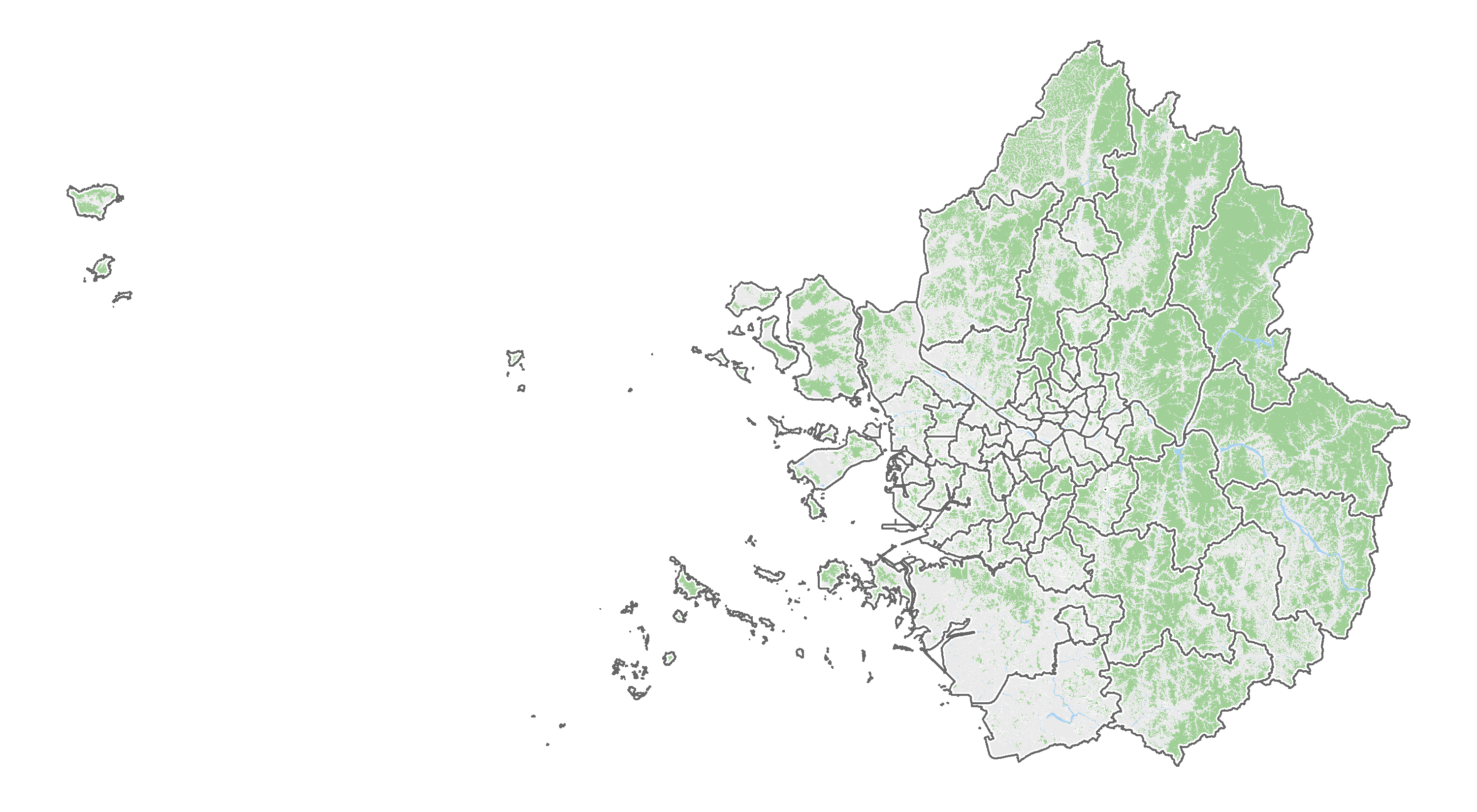
하나의 지도로 그리기

정리된 데이터를 기반으로 ggplot2 패키지를 사용해 지도를 그립니다. geom_sf 함수를 사용하여 각 데이터셋(행정구역, 녹지, 산지, 수계, 도로)을 별도의 레이어로 추가합니다. 시각적인 구분을 위해 채우기 색상(fill)과 경계선 색상(colour), 두께(size)를 지정합니다. 마지막으로, theme_void를 적용하여 축과 배경을 제거하고 데이터를 돋보이게 합니다.

ggplot() +
  geom_sf(data = sgg, colour=NA, fill="#eaeaea") + # 시군구 영역
  geom_sf(data = green, colour=NA, fill="#A0D097") + # 녹지
  geom_sf(data = mt, colour=NA, fill="#A0D097") + # 산지
  geom_sf(data = water, colour=NA, fill="#A5D1F2") + # 수계
  geom_sf(data = road, colour=NA, fill="white", linewidth=0.1) + # 도로
  geom_sf(data = sgg, colour="white", fill=NA, linewidth=1.3) + # 시군구 경계
  geom_sf(data = sgg, colour="gray40", fill=NA, linewidth=0.5) + # 시군구 경계
  theme_void()

---